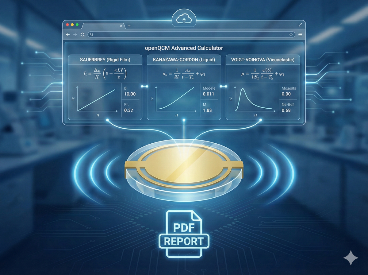

Three models. One interface. No installation. Today we’re releasing a tool we’ve wanted to build for a long time: a unified QCM calculator that covers the full range from rigid films in vacuum to viscoelastic layers in liquid — entirely in your browser.
If you work with QCM, you’ve almost certainly done this: opened a spreadsheet, typed in the Sauerbrey equation, double-checked the quartz constants, and hoped you didn’t make a sign error somewhere. For quick estimates, that works fine. But when you need to switch between models, compare regimes, or generate a clean report for a publication — it gets tedious fast.
The openQCM Advanced Calculator is our answer to that problem. It’s free, it runs entirely in the browser, and it’s available right now.
→ Launch the openQCM Advanced Calculator
Why a Unified Calculator
QCM is deceptively simple in principle — a mass on a vibrating crystal shifts the frequency — but the physics changes dramatically depending on what’s on the surface and what medium surrounds it.
A rigid metallic thin film in vacuum? Sauerbrey is all you need. A Newtonian buffer solution in a flow cell? You want Kanazawa-Gordon. A hydrated protein layer that’s neither fully rigid nor fully liquid? That’s Voigt-Voinova territory, and the equations get considerably more involved.
Most online tools cover only the first case. We wanted a single environment where all three models coexist with consistent notation, proper physical constants, and diagnostic guidance to help you decide which model applies to your experiment.
The Three Models
1. Sauerbrey — Rigid Film in Air or Vacuum
The foundational equation of QCM. For a thin, rigid, uniformly distributed film that oscillates in phase with the crystal, the frequency shift is directly proportional to the adsorbed mass per unit area:
\Delta f = -\frac{2 f_0^2}{A \sqrt{\rho_Q \mu_Q}} \, \Delta m
The calculator takes as input the fundamental frequency f0, the electrode diameter, the measured Δf, and the sample density ρf. From these it derives the mass sensitivity constant Cf, the film thickness, and the total mass change Δm.
It also computes the mass saturation limit and maximum sample thickness — useful checks to verify that your measurement stays within the validity range of the rigid-film approximation (|Δf|/f0 ≪ 1).
When to use it: Thin metallic films, oxide layers, self-assembled monolayers in air, any deposition where dissipation is negligible and Δf/n is approximately constant across harmonics.
Reference: G. Sauerbrey, Z. Phys. 155, 206–222 (1959)
2. Kanazawa-Gordon — Newtonian Liquid Loading
When one face of the crystal contacts a bulk liquid, the oscillating surface generates a shear wave that decays exponentially into the fluid. The result is both a frequency decrease and an increase in dissipation. Kanazawa and Gordon showed that for a semi-infinite Newtonian liquid:
\Delta f = -f_0^{3/2} \sqrt{\frac{\rho_L \eta_L}{\pi \rho_Q \mu_Q}}
The calculator supports two operating modes:
Forward mode. You provide the liquid density ρL and viscosity ηL. The calculator predicts Δf, the dissipation change ΔD, and the viscous penetration depth δ.
Inverse mode. You provide a measured Δf. The calculator extracts the product ρL·ηL and, given the density, the liquid viscosity.
The viscous penetration depth δ tells you how far the acoustic shear wave extends into the liquid — typically a few hundred nanometers at MHz frequencies. This is an important parameter: anything beyond δ from the surface is effectively invisible to the QCM.
Reference: K.K. Kanazawa & J.G. Gordon II, Anal. Chem. 57, 1770–1771 (1985)
3. Voigt-Voinova — Viscoelastic Film Analysis
This is where things get interesting. Many real-world films — polymer brushes, hydrogels, protein adlayers, DNA monolayers — are neither rigid nor liquid. They are viscoelastic: they store some energy elastically and dissipate the rest.
The Voigt-Voinova model treats the film as a Kelvin-Voigt element with a complex shear modulus:
G^* = G' + iG''
where G′ is the storage (elastic) modulus and G″ is the loss (viscous) modulus. The loss component can equivalently be expressed as a film viscosity: G″ = 2πfηf.
The calculator takes as input the film density, thickness, both modulus components, and — optionally — the bulk liquid properties (for films operating in liquid). It then predicts:
Frequency shift Δf and dissipation change ΔD
ΔD/|Δf| ratio — a diagnostic that helps distinguish rigid from viscoelastic films
Loss tangent tan(δ) = G″/G′ — classifies the film regime
Sauerbrey rigid-film limit ΔfS — for direct comparison with the full viscoelastic prediction
If Δf ≈ ΔfS and ΔD is small, your film is effectively rigid and Sauerbrey is sufficient. If they diverge significantly, viscoelastic effects dominate and a more complete model is required.
Reference: M.V. Voinova et al., Phys. Scr. 59, 391–396 (1999)
PDF Report Generation
Every calculation can be exported as a professional PDF report, ready for your lab notebook, a publication supplement, or a project deliverable.
Each report includes:
All input parameters and computed results, clearly tabulated
Proper mathematical notation — Δf, ρ, η, δ, G′, G″ rendered correctly
AT-cut quartz constants — ρQ, μQ, ZQ for reference
A didactic description of the model used, explaining the physics and input parameters
The original literature reference
The PDF engine is fully embedded — no external CDN dependencies, no network requests. It works offline, behind firewalls, and in restrictive IT environments. This was actually a non-trivial engineering challenge: the jsPDF library is inlined with a custom module-detection wrapper, and all mathematical symbols are rendered through an offscreen canvas to bypass the limitations of standard PDF fonts. But that’s a story for another blog post.
Design Principles
A few decisions we made deliberately:
Zero installation
Pure HTML/CSS/JavaScript. No backend. No account. No cookies. Your data stays on your machine.
Real-time feedback
Results update instantly as you type, so you can explore how parameters affect the output without hitting a “calculate” button.
Educational by default
Every PDF report explains the model, not just the numbers. Useful for teaching, for onboarding new lab members, and for your own reference.
Built with AI, Guided by Physics
In the spirit of openness that defines the openQCM project, we want to share how this tool came to life.
The openQCM Advanced Calculator was developed in close collaboration with Claude, Anthropic’s AI assistant. Claude contributed to the interface design, the implementation of the three physical models, the self-contained PDF export engine, and the didactic descriptions that accompany each report.
The process was not “we told an AI to make a calculator.” It was a genuine iterative dialogue — domain expertise driving the physics, the AI handling the implementation, and constant back-and-forth to refine both. We tested every formula against known analytical solutions and reference papers. The result is something neither side would have built alone, and we think it represents an interesting model for developing scientific tools.
We mention this not as a marketing exercise, but because we believe transparency about methods matters — in science and in engineering alike.
We Want Your Feedback
This calculator is a starting point, not a finished product. It covers the three foundational QCM models, but QCM science is much broader than that. We have ideas for future development, but what matters most is what you need in your lab.
Are there additional models you would like us to implement? Multi-overtone Sauerbrey fitting, Kelvin-Voigt parameter extraction from multi-harmonic data, BVD equivalent circuit analysis?
Would new features be useful? Data import/export, graphical parameter sweeps, comparison between models on the same dataset?
Did you find something that doesn’t look right? An edge case, an unclear label, a unit conversion that seems off?
Every suggestion from the research community helps us make the tool better for everyone. Please share your thoughts through the openQCM Forum or contact us directly.
Try It Now
The openQCM Advanced Calculator is free, open, and ready for your next experiment:
→ openqcm.com — QCM Advanced Calculator
We hope it saves you some spreadsheet headaches and becomes a useful companion at the bench. Happy measuring.
Questions, feature requests, or bug reports? We’d love to hear from you — get in touch or join the conversation on the openQCM Forum.