
Ever wondered what really happens when your openQCM measures dissipation? Today we’re opening the hood and showing you exactly how it works—including the engineering challenge that made us rethink the standard approach.
One of the questions we get asked most often is: “How exactly does the dissipation measurement work?”
It’s a fair question. And honestly, the answer involves a bit of creative problem-solving that we think you’ll find interesting—especially if you’ve ever struggled with measurements in viscous solutions or wondered why your higher overtones sometimes behave unexpectedly.
The Sensing Principle
openQCM Q-1 and openQCM NEXT measure two parameters simultaneously: frequency (related to mass changes) and dissipation (related to viscoelastic properties). This dual measurement capability is what makes QCM-D such a powerful technique for characterizing soft matter, biological films, and polymer layers.
Unlike systems based on oscillator circuits or the ring-down technique, our instruments employ a scalar network analyser approach. We passively interrogate the quartz crystal by performing a frequency sweep around the resonance, generating a sinusoidal signal and measuring the amplitude of the crystal’s response.
Think of it as gently probing the system across a range of frequencies rather than forcing it to oscillate at a predetermined point. This approach allows us to reconstruct the complete resonance curve and extract both frequency and bandwidth information.
Building the Resonance Curve
The measurement process is conceptually straightforward:
Step 1. Set an excitation frequency f₁ and measure the response amplitude
Step 2. Increment to f₂, f₃, f₄… measuring each response
Step 3. The complete set of points defines the resonance curve
Step 4. Repeat for each harmonic: fundamental, 3rd, 5th, 7th overtone…
From this curve, we extract the resonance frequency (the peak position) and the bandwidth (the peak width), which is directly related to energy dissipation in the system.
The Classical Approach: −3 dB Bandwidth
The standard definition of dissipation is elegantly simple:
D = \frac{1}{Q} = \frac{\Delta f}{f_r}
where Δf is the bandwidth measured at the −3 dB level (half-power points), corresponding to an amplitude of Apeak/√2. This definition has solid physical grounding: it relates directly to the energy dissipated per oscillation cycle.
In an ideal world, this would be all we need. However, real-world measurements—particularly at higher overtones—present a challenge that isn’t always discussed in textbooks.
The Overtone Problem
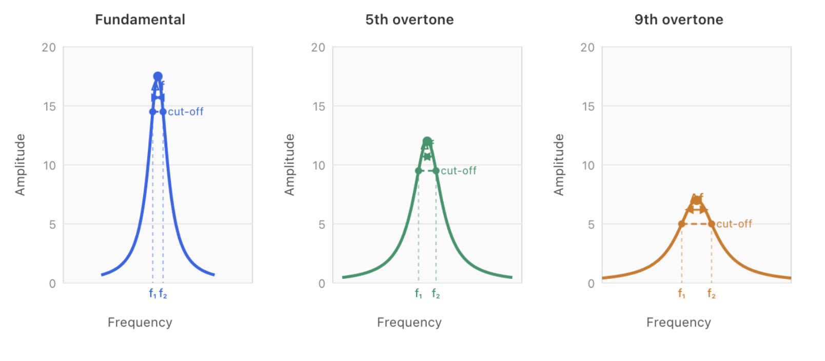
During extensive testing of our instruments, we observed something important: the amplitude of resonance peaks decreases significantly as the overtone order increases.
If your fundamental at 10 MHz shows a peak amplitude of 18 arbitrary units, the 5th overtone might reach only 12–14 units, and the 9th overtone even less. This occurs due to several physical

factors:
- Reduced mechanical displacement at higher harmonics
- Frequency-dependent coupling efficiency between electronics and crystal
- Increased energy losses at higher frequencies
When the peak amplitude becomes s
ufficiently low, the standard −3 dB approach encounters practical difficulties:
Noise floor proximity. The −3 dB cut-off level approaches the system noise, making precise identification of f₁ and f₂ difficult.
Degraded signal-to-noise ratio. Small fluctuations translate into significant bandwidth errors.
Undefined intersections. In extreme cases, the −3 dB level may not clearly intersect the resonance curve at all.
If you’ve ever experienced unstable dissipation readings at higher harmonics, this is likely the underlying cause.
Our Approach: Adaptive Cut-off Levels
Faced with this limitation, we had two options: accept that higher overtones would be inherently unreliable, or develop a more robust methodology. We chose the latter.
openQCM Q-1 and openQCM NEXT employ a custom cut-off level for each harmonic, defined as:
A_{cutoff,n} = A_{peak} - \Delta A_n
where ΔAn is an amplitude offset calibrated for each overtone during instrument setup, ensuring the measurement remains well above the noise floor while still capturing the relevant portion of the resonance curve.
The ΔAn values are determined during instrument calibration, optimized for each harmonic to balance noise immunity with measurement sensitivity.
Physical Interpretation
We want to be transparent about what this methodology means for your data.
The parameter we measure—denoted Dn(inst) (instrumental dissipation)—is systematically related to, but not numerically identical to, the canonical dissipation factor defined at −3 dB. The absolute values will differ.
However, and this is the key point:
Relative variations ΔDn(inst) faithfully track real changes in energy dissipation. When your film softens, D increases. When it rigidifies, D decreases. The trends are physically meaningful and reproducible—which is precisely what matters for real-time monitoring experiments.
For applications requiring absolute comparison with literature values, correction factors can be applied to map the measured bandwidth to the equivalent −3 dB value. This mapping depends on the resonance lineshape and can be determined analytically for Lorentzian resonances or empirically using reference measurements.
Multi-Harmonic Analysis
One of the strengths of QCM-D is the ability to probe your sample at multiple frequencies simultaneously. Different overtones are sensitive to different effective depths within the contacting medium:
Lower Harmonics
Greater penetration depth. Sensitive to the bulk properties and entire film thickness.
Higher Harmonics
Smaller penetration depth. More sensitive to surface and near-surface layers.
Comparing dissipation across harmonics provides insight into the vertical structure of your film. Is it homogeneous throughout? Does the surface behave differently from the bulk? Multi-harmonic data helps answer these questions.
Rigidity Verification
For rigid films where the Sauerbrey equation applies, you should observe:
- Δfn/n approximately constant across all harmonics
- Dn values remaining low and relatively constant
Significant deviations from this behavior—particularly D values that increase with overtone number—indicate viscoelastic contributions that require more sophisticated modelling approaches such as the Voigt or Maxwell models.
Practical Recommendations for Viscous Solutions
Based on our experience supporting researchers across diverse applications, here are some practical suggestions for working with high-viscosity samples:
Widen the frequency sweep range. Viscous loading significantly broadens the resonance peak. Ensure your sweep captures the complete curve, including the tails.
Increase the number of sampling points. Higher point density improves the accuracy of peak detection and bandwidth determination, particularly for broad, low-amplitude resonances.
Prioritize lower harmonics. The fundamental and 3rd overtone typically provide the most reliable signal in viscous environments, where higher overtones may be strongly attenuated.
Summary
openQCM Q-1 and openQCM NEXT measure dissipation by reconstructing the resonance curve through frequency sweeps and calculating the bandwidth for each harmonic.
Our adaptive cut-off methodology addresses a practical limitation of the standard −3 dB approach: the reduced signal amplitude at higher overtones. By using harmonic-specific cut-off levels calibrated above the noise floor, we ensure reliable dissipation measurements across all available overtones.
Is this a departure from the canonical definition? Yes. Does it provide meaningful, reproducible, physically relevant data for monitoring viscoelastic changes in real-time? Absolutely.
The multi-harmonic dissipation data, combined with frequency shift measurements, enables characterization of soft films, hydrated layers, and biological samples where the Sauerbrey equation alone is insufficient.
Questions about our measurement methodology or need assistance optimizing your experimental setup? We’re always happy to discuss—get in touch or leave a comment below.